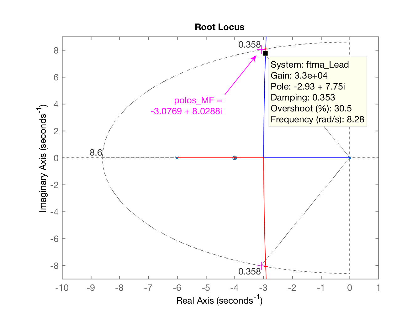
Exemplo de Projeto de Lead usando Contribuição angular.

Aula de 09.06.2021

Uso do script angulos3.m $+$ arc.m.

Exemplo: Projete um compensadores por avanço de fase que reduza $t_s$ por 2 enquanto mantêm sobressinal abaixo de 30% (baseado no example 9.4 de NISE):

Sintonizando um controlador proporcional para este sistema de forma à respeitar $\%OS \le 30\%$, se descobre o valor: $K=60,5267$ com o qual se obtêm em MF: $t_s=3,8778$ segundos. Então o novo $t_s’=1,2926$.

Comandos no Matlab:

Note:

1) angulos3.m deve ser acompanhado da função: arc.m para poder funcionar!

2) Para usar angulos3.m já deve estar disponível a avariável G (uma tf que corresponde a transfer fucntion da planta: $G(s)$) no ambiente de trabalho do Matab (Workspace):

>> help angulos3
  programa para Projeto de Lead atrav��s de
  contribui����o angulas
  Fernando Passold, em 23/11/2019, revisado em 30/05/2020
  Baseado em "example_9_4.m" de /UCV/Control/ (2009)
  Lead Compensator Desing (NISE)
 
  Exige como entrada (para funcionar), as seguintes vari��veis:
 
  G=tf( , )
 
  Gera texto na tela compat��vel com Markdown
​
>>

Caso se interesse você pode tentar entender o código usando:

>> edit angulos3.m

Note: se você tentar executar angulos3.m sem existir a variável G, teremos um erro:

>> angulos3
​
## Lead Controller Design
​
In this version you should arbitrate the initial position of the ZERO of C(z)
​
Plant (in s-plane) informed, G(s):
​
```matlab Undefined function or variable 'G'.
​
Error in angulos3 (line 27)
zpk(G)
 
>>

Então, iniciando este projeto, informando a planta, temos:

>> G = tf ( 1, poly( [0 -4 -6] ) )
​
G = 
           1
  -------------------
  s^3 + 10 s^2 + 24 s
 
Continuous-time transfer function.
​
>> zpk(G)
 
        1
  -------------
  s (s+6) (s+4)
 
Continuous-time zero/pole/gain model.
​
>> angulos3

O que gera:

Lead Controller Design

In this version you should arbitrate the initial position of the ZERO of C(z)

Plant (in s-plane) informed, G(s):

ans =
 
        1
  -------------
  s (s+6) (s+4)
 
Continuous-time zero/pole/gain model.

Maximum overshoot desired (%OS), in %: ? 30

The damping factor should be: $\zeta = 0.3579$

Enter desired settling time, $t_s$: ? 1.3

It results in the natural oscillation frequency, $w_n = 8.5982$ (rad/s)

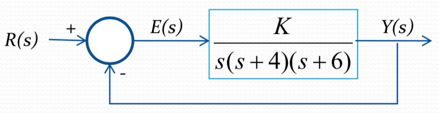
The MF poles (in the s-plane) should be located in: $-3.0769 \pm j8.0288$

Enter the position of the controller ZERO ($z_c = 0.0000$): ? -4

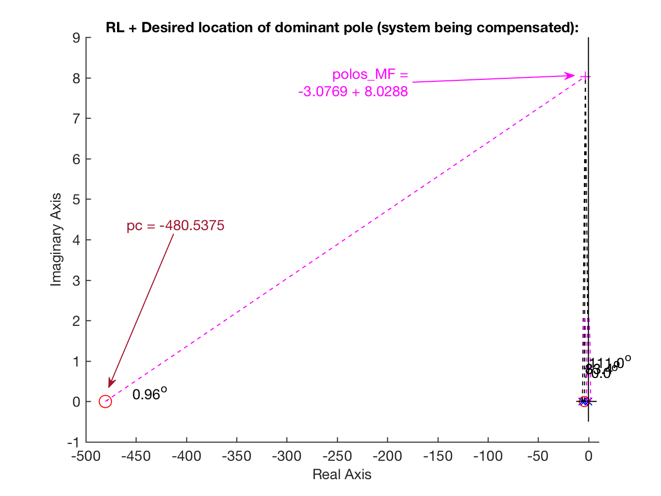
C_aux =
​
  s + 4
  
Continuous-time transfer function.  

Angular contribution of each pole in the s-plane:

$p_1 = 0 \rightarrow 110.97^{o}$ $p_2 = -6 \rightarrow 69.99^{o}$ $p_3 = -4 \rightarrow 83.44^{o}$

Sum of angular contribution of poles, $\sum {\theta_{\text{P��los}}} = 264.40^{o}$

Angular contribution of each zero in the s-plane:

$z_1 = -4 \rightarrow 83.44^{o}$

Sum of angular contribution of zeros, $\sum {\theta_{\text{Zeros}}} = 83.44^{o}$

Final angle for the pole of $C(s)$, $\theta_{z_{c}} = 0.9634^o$

Final position for the Lead pole: $p_c=-480.5375$

The Lead controller final result is (variable C_Lead):

ans =
 
    (s+4)
  ---------
  (s+480.5)
 
Continuous-time zero/pole/gain model.

The $FTMA(s)$ (variable ftma_Lead):

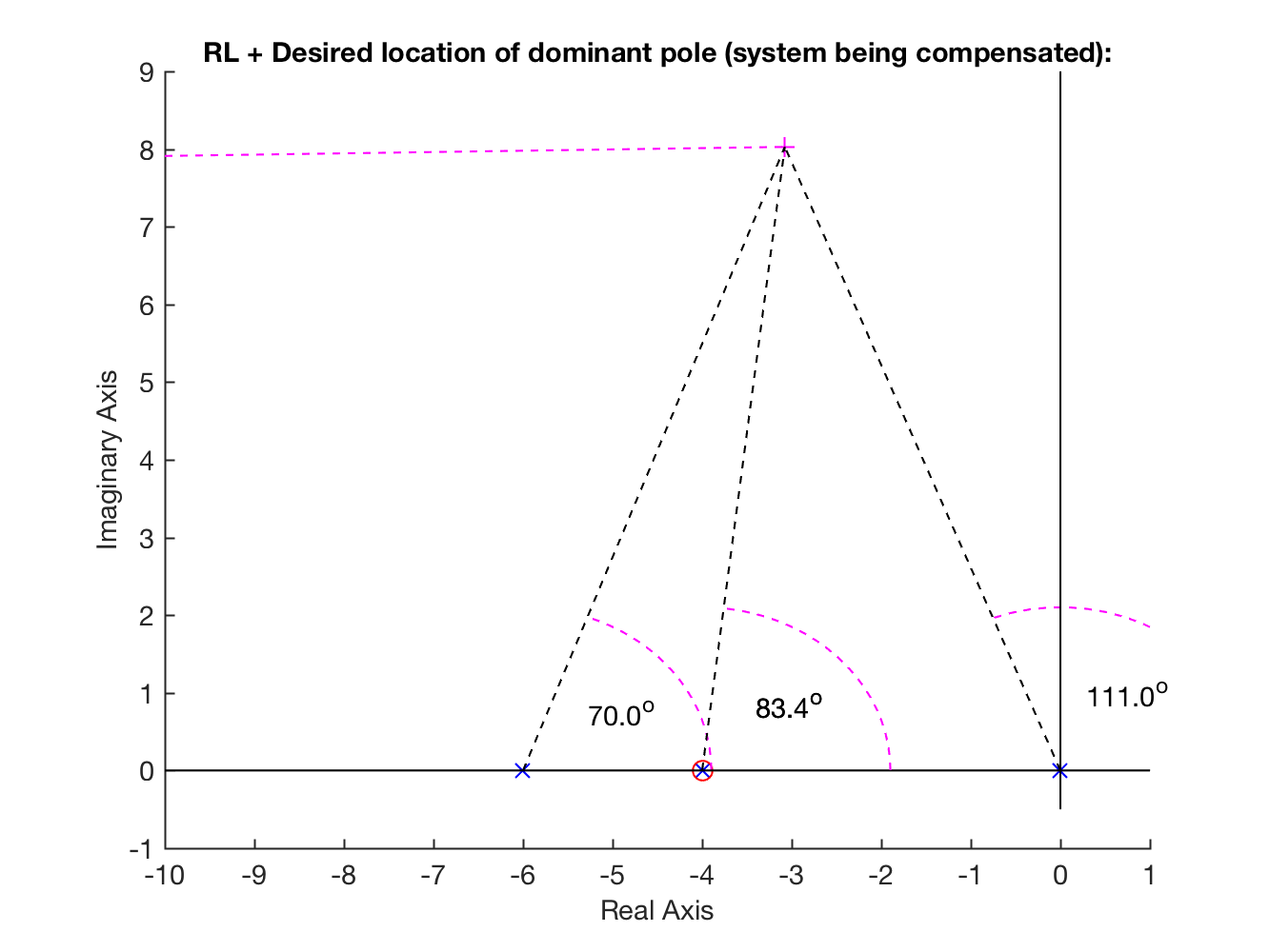
ans =
 
           (s+4)
  -----------------------
  s (s+480.5) (s+6) (s+4)
 
Continuous-time zero/pole/gain model.

Final RL graph:

Fim do script, Favor observar janelas gráficas...

Ajeitando os gráficos gerados:

xxxxxxxxxx
>> figure(1); axis([-10 1 -1 9]) % No gráfico mostrando contribuições angulares

Gráfico sem zoom:	Gráfico ajustado (zona de interesse):

Note que com o ajuste anterior, não se percebe o pólo deste controlador defindo em $s=-480$ (bastante distante dos outros pólos e zeros da $FTMA(s)$).

Ajustando a segunda janela gráfica (já com o RL da $FTMA(s)$ incluindo eq. completa do Lead):

xxxxxxxxxx
>> axis([-10 1 -9 9])

resulta em:

Continuando com o projeto iniciado por angulos3.m (note que este script não determina o ganho necessário para o controlador, apenas termina com o gráfico do RL pronto para definição do ganho do mesmo):

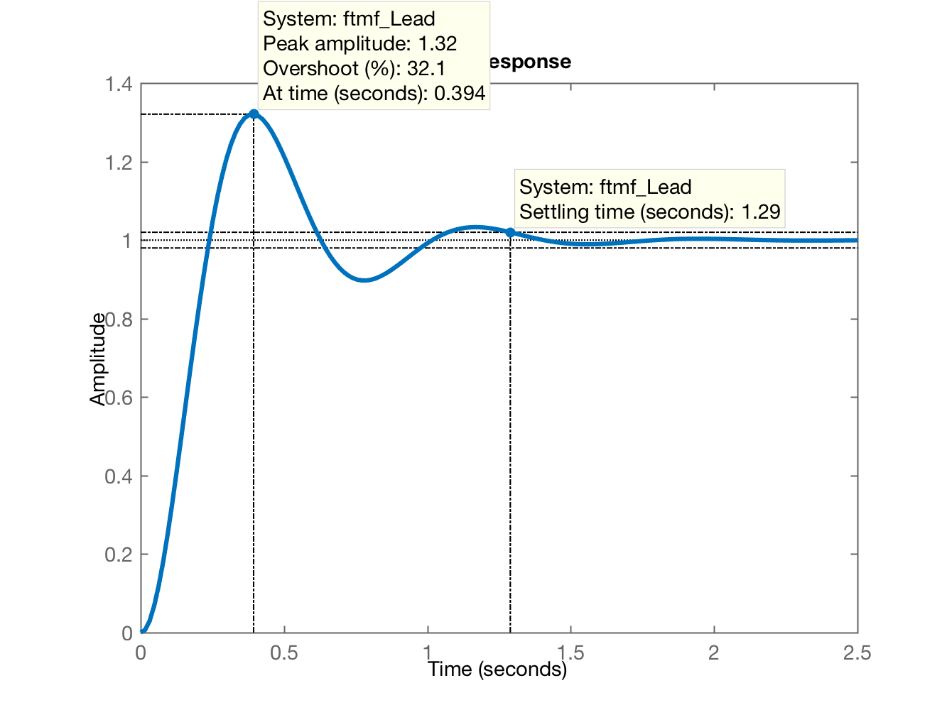
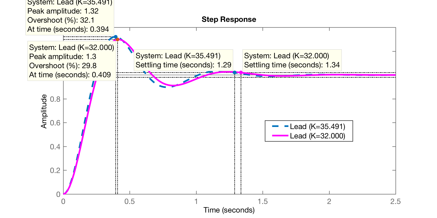
xxxxxxxxxx
>> [K_Lead, polosMF] = rlocfind (ftma_Lead)
Select a point in the graphics window
selected_point =
  -2.9230 + 8.0805i
K_Lead =
   3.5491e+04
polosMF =
   1.0e+02 *
  -4.8069 + 0.0000i
  -0.0292 + 0.0808i
  -0.0292 - 0.0808i
  -0.0400 + 0.0000i
>> % fechando a malha
>> ftmf_Lead = feedback(K_Lead*ftma_Lead, 1);
>> figure; step(ftmf_Lead)
>> ftmf_Lead2 = feedback(32000*ftma_Lead, 1); % ajustando ganho para reduzir algo o %OS
>> figure; step(ftmf_Lead, ftmf_Lead2)
>> legend('Lead (K=35.491)', 'Lead (K=32.000)')

E temos então 2 gráficos:

E o gráfico que compara com o mesmo Lead mas com ganho reduzido para $K_{Lead}=32000$, de forma a manter o $\%OS \le 30\%$:

Fim.

Fernando Passold, em 09.06.2021